In this example, we will create a new high-resolution seafloor to use with the dave simulation.

You can run the example world using only the basic dave installation requirements. To run through the full tutorial or create your own seafloor, you will need to install gdal and proj:

sudo apt-get install gdal-bin
sudo apt-get install proj-bin

Todo: Verify whether we need to install proj for the basic tutorial. Recommend installation regardless but not all gdal functions will require it.

This tutorial is not sensitive to gdal and proj versions, as long as they are mutually compatible, but many other operations do require specific versions. We recommend proceeding with caution before upgrading either of these software packages on your system.

If you normally run dave in the docker environment, you can launch a terminal with gdal and proj already installed via:

docker pull woensugchoi/bathymetry_converter:release && docker run -it --rm -v $PWD:/home/mkbathy/workdir -w /home/mkbathy/workdir woensugchoi/bathymetry_converter:release bash

Building a Usable Dataset

First, we’ll need to find or create a dataset that will represent the seafloor. See the Bathymetry Converter tutorial for some suggestions on where to get real bathymetry, or you can build your own file using 3D modeling software. The data need to be in a format that is readable by gdal - see the GDAL website for a discussion of types. Some manipulation will be needed to work with other formats.

Here’s an example using bathymetry data from the Santorini Island area.

For this example, we will use the region around Santorini Island, available from EMODNet. On the “downloads” sidebar, click on “High resolution areas” and find the appropriate area to download. This site uses a proprietary format, .emo, that is not currently supported by GDAL. Fortunately, the format can be read as a .csv and manually manipulated into the supported XYZ raster format with little effort. We just extract the longitude, latitude, and average depth fields and label the appropriate columns as X, Y, Z. Since the depth dimensions were given as positive values and the Z input needs to be an elevation, we also need to swap the signs on the Z column values. We’ll save this as 269_Santorini.csv.

Prepping for Gazebo Import

Heightmaps in Gazebo need to be of dimensionality (2ⁿ + 1) x (2ⁿ + 1), where n is an integer, because of the requirements of the rendering engine. We’ll need to rescale the input to comply with this. In the case where the input data file is not square, we can stretch the heightmap when importing it to Gazebo, but this will give us different resolutions in the two dimensions.

We can fill in any gaps in the data and convert it to a usable heightmap with GDAL. There are several useful functions that can do this. For this data, we’ll fill in the missing points with gdal_fillnodata.py 269_santorini.csv smooth0.tif. Inspecting the results of this operation via gdalinfo smooth0.tif gives: ```Driver: GTiff/GeoTIFF Files: smooth0.tif Size is 1424, 1056 Origin = (24.983333333334507,36.683333336668248) Pixel Size = (0.000520833330991,-0.000520833336493) Image Structure Metadata: INTERLEAVE=BAND Corner Coordinates: Upper Left ( 24.9833333, 36.6833333) Lower Left ( 24.9833333, 36.1333333) Upper Right ( 25.7250000, 36.6833333) Lower Right ( 25.7250000, 36.1333333) Center ( 25.3541667, 36.4083333) Band 1 Block=1424x1 Type=Float32, ColorInterp=Gray NoData Value=-32768

What we have created is a rectangular image with equally spaced pixels.  We will use this file size to resize the heightmap on import and to choose our dimensions for the next step.

Finding the right scale for the data is important - if we oversample, we end up with a pixelated look (think Minecraft).  If we undersample, we aren't taking full advantage of the richness of the input data.

The original Santorini dataset contains roughly one million data points, covering an area of 60 square km.  If the points were evenly distributed, this would give an approximate resolution of 60 meters.

We'll choose 1025 x 1025 as a starting point, as this is the closest viable match to the file size we found with the call to gdalinfo.  Via `gdalwarp -ts 1025 1025 smooth0.tif Santorini_heightmap.tif` we create a  file that is ready to import into Gazebo.

For more information on importing heightmaps, see the Gazebo [DEM tutorial](http://gazebosim.org/tutorials/?tut=dem).

## Creating the Model SDF

There are two fields we’ll want to play with in the sdf.  First, we need to scale the heightmap appropriately for our world.  If we wanted to maintain some level of geographic accuracy, we would figure out the true spatial extent of the grid in meters, and use that information to populate the <size> field.  For this example, we want to simulate higher-resolution data, so we’ll scale everything down by a rough factor of ten.  We’ll also adjust the <pos> field to position the heightmap more or less where we want it relative to our Gazebo world coordinate system.

Finally, we can add a simple texture to make the seafloor more interesting.  Here's the sdf snippet that adds the seafloor into the world:

<model name="heightmap">
  <static>true</static>
  <link name="link">
    <collision name="collision">
      <geometry>
        <heightmap>
            <uri>file://media/Santorini_heightmap.tif</uri>
            <!-- Scale for original size of terrain segment -->
            <size>8090 6000 141</size>
            <pos>0 0 1400</pos>
        </heightmap>
      </geometry>
    </collision>
    <visual name="visual">
      <geometry>
        <heightmap>
          <texture> <!-- Add sample texture for visualization -->
            <diffuse>file://media/materials/textures/dirt_diffusespecular.png</diffuse>
            <normal>file://media/materials/textures/flat_normal.png</normal>
            <size>1</size>
          </texture>
          <uri>file://media/Santorini_heightmap.tif</uri>
          <size>8090 6000 141</size>
          <pos>0 0 1400</pos>
         </heightmap>
      </geometry>
    </visual>
  </link>
</model> ```

To improve performance of the physics engine with very high resolution data, it may be helpful to use a lower resolution heightmap for the collision element. We don’t need to do this for our ~6 meter resolution file.

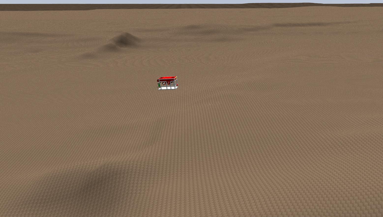
To run this example: roslaunch dave_demo_launch dave_new_environment.launch