Demonstration of DVL Water Tracking and Current Profiling

Prerequisites

• The Ocean Current tutorial discusses the model used for specifying the ocean current velocity.

Setup

Launch simulation

roslaunch dave_demo_launch dave_current_profiling_demo.launch

The simulation will spawn a single Teledyne WHN DVL at a position approximately 15 meters beneath the water’s surface. Initially the water current is zero but can be adjusted using ROS services.

The DVL publishes the following messages:

• The Dvl.msg provides a single velocity solution in the sensor’s frame using either bottom tracking or water tracking (if enabled).
• The Adcp.msg provides current profile information for a series of depth cells in the DVL’s beam pattern. Current profile can be provided in either beam-specific coordinates (four solutions per depth cell) or vehicle-specific coordinates (one solution per depth cell).

A simple current profiling verification test

1. Start the simulation
2. Plot the water velocities in beam coordinates rosrun rqt_plot rqt_plot /dvl/dvl_current/vel_bin_beams[0]/velocity_bin_beam[0] to plot the beam-specific x, y, and z current velocities for the first cell (nearest the instrument) of the first beam. Data from other cells can be plotted by changing the velocity_bin_beam index, and data from other beams can be plotted by changing the velocity_bin_beams index.
3. Make a step change in water current velocity at layer 2 (when loaded, the DVL’s first depth cell is centered at approximately 19.5m), e.g., rosservice call /hydrodynamics/set_stratified_current_velocity '{layer: 2, velocity: 1.0}'
4. Wait a few seconds, then change the layer 2 velocity to zero, e.g., rosservice call /hydrodynamics/set_stratified_current_velocity '{layer: 2, velocity: 0.0}'
5. Afert a few seconds, change the layer 2 velocity to its original value, e.g., rosservice call /hydrodynamics/set_stratified_current_velocity '{layer: 2, velocity: 1.8}'

1. Change the horizontal direction of the current at layer 2, e.g., rosservice call /hydrodynamics/set_stratified_current_horz_angle '{layer: 2, angle: 1.570796}'
2. Change the vertical direction of the current at layer 2, e.g., rosservice call /hydrodynamics/set_stratified_current_vert_angle '{layer: 2, angle: 0.523599}'
3. Repeat steps 2 through 7 as desired for different beams, depth layers, current directions, and current speeds to observe profiling performance in different situations.

Implementation

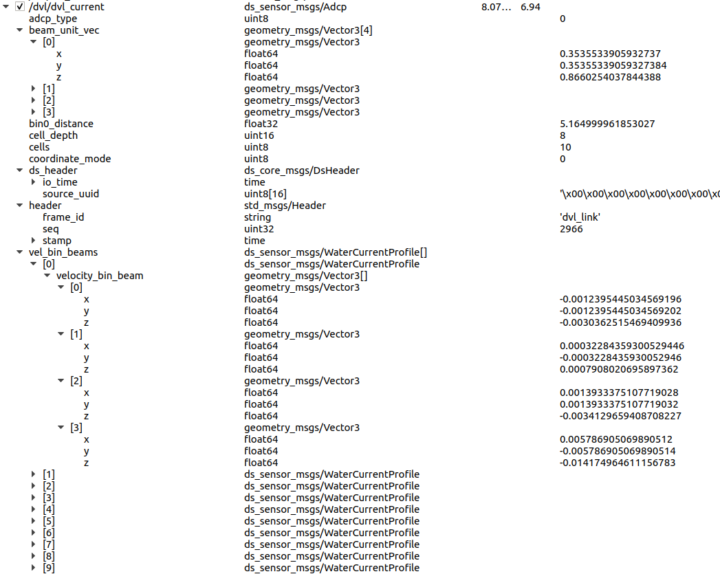
By default, the DVL current profiling information is published in beam-specific coordinates. Beam-specific velocities are computed using the beam unit vectors, which are also published in the Adcp message. The beams for the Teleyne WHN DVL are oriented 30^o from vertical at 45^o, 135^o, 225^o, and 315^o relative to the sensor. With this orientation, the X and Y components of the beams 0 and beam 2 unit vectors will be the same, and the same components of the beam 1 and 3 unit vectors will be inverses. The computed X and Y velocities for each beam will be the same for beams 0 and 2 and opposite for beams 1 and 3.

Beams that are in contact with the bottom will not compute a current velocity beyond the last no-contact depth cell. In the demonstration simulation, beams 3 and 4 are within range of the bottom, so their velocity solutions for the furthest depth cell will be 0.

The plugin can be set to publish current profiling information in instrument-specific coordinates by changing the value of the currentProfileCoordMode to 1 as indicated in the following sensor element from the Teledyne WHN model SDF file.

<sensor name="dvl_sensor" type="dsros_dvl">
  <always_on>1</always_on>
  <update_rate>7.0</update_rate>
  <plugin name="dvl_sensor_controller" filename="libdsros_ros_dvl.so">
    <robotNamespace>dvl</robotNamespace>
    <topicName>dvl</topicName>
    <rangesTopicName>ranges</rangesTopicName>
    <frameName>dvl_base_link</frameName>
    <pointcloudFrame>dvl_base_link</pointcloudFrame>
    <updateRateHZ>7.0</updateRateHZ>
    <gaussianNoiseBeamVel>0.005</gaussianNoiseBeamVel>
    <gaussianNoiseBeamWtrVel>0.0075</gaussianNoiseBeamWtrVel>
    <gaussianNoiseBeamRange>0.1</gaussianNoiseBeamRange>
    <minRange>0.7</minRange>
    <maxRange>90.0</maxRange>
    <maxRangeDiff>10</maxRangeDiff>
    <beamAngleDeg>30.0</beamAngleDeg>
    <beamWidthDeg>4.0</beamWidthDeg>
    <beamAzimuthDeg1>-135</beamAzimuthDeg1>
    <beamAzimuthDeg2>135</beamAzimuthDeg2>
    <beamAzimuthDeg3>45</beamAzimuthDeg3>
    <beamAzimuthDeg4>-45</beamAzimuthDeg4>
    <enableWaterTrack>1</enableWaterTrack>
    <waterTrackBins>10</waterTrackBins>
    <currentProfileCoordMode>1</currentProfileCoordMode>
    <pos_z_down>false</pos_z_down>
    <collide_bitmask>0x0001</collide_bitmask>
  </plugin>
  <pose>0 0 0 0 0 0</pose>
</sensor>

When computing the current profile in the instrument frame, a separate velocity solution is computed for each depth cell and published in the Adcp message /dvl/dvl_current/vel_bin_beams[0] field. The solution is computed as a least-squares solution of the 4x3 matrix of individual beam velocities (including added noise). If any beam is in contact with the bottom, no solution will be computed for the affected depth cells. Since beams 3 and 4 are in contact with the bottom in the demonstration simulation, the velocity solution for the last depth cell is 0.